Your connection to advanced PCB manufacturing
Historically PCB fabrication and delivery of finished products preceded test methods to validate the PCBs. In the 1970’s PCBs were fabricated and shipped without electrical test validation. Mania brought electrical testing to the industry and soon after electrical testing became standard and a requirement for all but the simplest products.
For the next decade PCBs were built by using a “Golden” board programming. The Golden board method used a finished PCB from a finished lot of PCBs and placed on a test fixture, an operator would place the PCB on a tester and initiate a self-learned shorts and opens program from the board. If the second PCB matched the first, a Golden board was established. One of the short comings of the Golden board testing however, is that it is susceptible to missing errors in the supplied fabrication data. The Golden board method would also allow for CAM errors to go undetected up to assembly. The solution finally came when CAM and net compare was made available in the late 1980s. Software was used to validate the received data before fabrication started, the same software was then used to generate an ET program to validate the finished PCB. This method saved product cycle time, prevented the loss of material, and saved manufacturing time at both PCB fabrication and assembly.
The same experience could be said about TDR, and AOI program downloading.
Today the industry is facing the challenge regarding microvia reliability, especially after the reflow of the PCB at assembly, during rework or operating in the field. As with electrical testing in the past, the industry designed PCBs using microvias without evaluating the thermal properties of the material or the geometries in the design. Fabricators produced the finished goods and evaluated the finished PCB to established standards such as IPC-6012. When difficult-to-detect failures occurred post-assembly a test method IPC-TM-650 2.6.27 was established and a caution was added to IPC-6012 rev in section 3.6 Structural Integrity. The testing of a D coupon via IPC-TM-650 2.6.27 did validate that the finished PCBs were safe for assembly, but it did not stop a fabricator from building a bad design. However, until now, there wasn’t a method to simulate a PCB design that validated that the material selection, dielectric thickness, microvia size, and configuration (single, stacked, or staggered microvias) could survive 6x reflows.
As with the evolution of electrical test and the use of the software to validate the design and the final test, we now have software that will validate the structural integrity of a microvia in a design before a PCB stack-up has been approved and implemented into the fabrication process. Our industry now has the opportunity to validate the design, fabricate a microvia design with confidence, and validate that the PCB has met the structural requirements by OM testing to IPC-TM-650 2.6.27.
For more information, listen to Gerry Partida on Altium’s podcast, Design Reliable Multiple Stack Microvias Like a Pro (altium.com).
Electric Field
Before discussing what is an electric field, let’s look to the Earth’s gravitational field for general answers about fields.
Gravitational Field
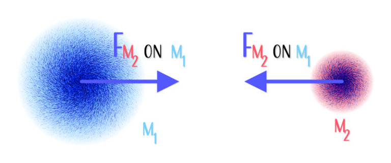
When we think of gravity, we tend to think of common objects falling towards Earth’s surface. But that is only half of an interaction. We do not tend to think about the Earth’s attraction to everyday objects because the Earth’s acceleration towards that object is imperceptibly small.
And we certainly don’t think about everyday objects exerting a gravitational force on one another, and that is because the gravitational interaction is so weak we have personally never witnessed it. Outside of carefully-designed experiments, you generally need an astronomically-sized object to generate the forces required to observe an interaction.
Do the Math
Use the gravitational mass of two objects, the constant of proportionality G, and the distance between the objects’ centers of mass, we can find the gravitational force of attraction between the objects. To do the math properly, we should consider the mass and exact location of every oil and mineral deposit, every rock, every wave, every person, and every other object in the Earth and on the surface. But that is too much work, so we assume a homogenous sphere.
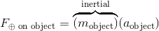
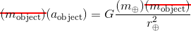
All humans near the surface of the Earth, from miners below the surface to pilots in commercial airplanes experience this same acceleration towards the center of the Earth. It is far easier to work with g=9.8(m/s2) than to go through this derivation every time you want to determine the acceleration of a new object. Since the mass of the object always cancels out of the equation, the acceleration will always be around g=9.8(m/s2).
The Earth is not homogeneous, and it’s not a sphere. It is an ellipsoid with mountains and valleys, oil and mineral deposits, oceans, and all sorts of unique features. The gravitational field surrounding the Earth is non-uniform.
Suppose you dropped an object at 800 equally spaced locations around the globe and drew an arrow at that location to indicate the direction of acceleration. In that case, you might end up with the image below.
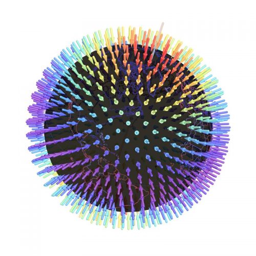
Vector Fields
If the length of the arrow is proportional to the magnitude of acceleration, the arrow becomes a vector. Mathematically, the collection of vectors is a vector field, and a value is defined everywhere in the region, not just the locations defined by arrows.
Fields are mathematical constructs that show how an object’s properties change in a two or three-dimensional region.
Since the vector-field we used in our example is due to gravity, another name for the collection of arrows is a gravitational field.